Why I Stopped Trusting Gut Feel
May 2026. We are eighteen months past the rollout of Google's Meridian core update, two years past the widespread adoption of AI Overviews for informational queries, and most SEO teams I talk to are still measuring topical authority the same way they measured it in 2021: a vague wave of the hand toward "content clusters" and a screenshot of their Domain Rating. I was one of those people until about fourteen months ago.
The moment that changed things was embarrassingly mundane. A client site I had been working on for two years had 340 published articles across a single vertical. A competitor with 61 articles was outranking them across the board. Not on a few keywords. Not just the hard ones. Across the board. Our DR was 54; theirs was 38. Our content calendar had been meticulously planned around pillar pages and supporting clusters. Theirs looked, from the outside, almost random.
That is when I understood I had no actual way to measure what was happening. I had intuitions. I had models. I had metaphors borrowed from other people's blog posts. What I did not have was a number, a repeatable process, or any honest answer to the question: how topically authoritative is this site, really?
Three attempts followed. All three taught me something. None of them worked cleanly on the first try.
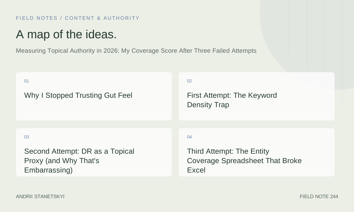
First Attempt: The Keyword Density Trap
My first pass at building a topical authority measurement system, sometime in the spring of 2025, was naive in a specific and instructive way. I pulled every ranking keyword for the site from Search Console and from a third-party rank tracker, de-duplicated them, and tried to build a "topic coverage percentage" by grouping keywords into clusters using a manual taxonomy I had built in a spreadsheet.
The taxonomy had 14 top-level categories and 87 subcategories. It took me and a content strategist about three weeks to build. It covered, we estimated, roughly 80 percent of the keyword universe for the vertical.
Then I tried to calculate coverage score as: (number of ranking URLs per subcategory) / (estimated total subtopics in subcategory). Simple ratio. Normalized to 100.
The problem appeared within the first week of using it. Coverage scores were inflating because a single URL that ranked for 40 keyword variations of the same underlying question was counting as 40 subtopics covered. I was measuring keyword breadth, not topic depth. A page titled "what is [topic]" that ranked for 40 long-tail variants of the same question would score identically to 40 genuinely distinct pages covering 40 distinct subtopics. That is not topical authority. That is just a popular page.
Scrapped it.
Second Attempt: DR as a Topical Proxy (and Why That's Embarrassing)
The second attempt is the one I am most reluctant to admit publicly, but it is also the most educational, so here it is.
After reading about topical PageRank as a concept, I got excited about the idea that link signals could approximate topical authority if you filtered them correctly. The logic was: if a site receives a high proportion of its inbound links from domains that are themselves authoritative specifically within a given topical space, that ratio should proxy for how much topical trust has been transferred.
I built a system that pulled referring domains, then used a third-party topic classification API to categorize each referring domain, then calculated what percentage of a site's inbound links came from domains in the same primary topic category. I called this "topical link concentration" and ran it across about 60 sites.
The results were interesting but almost entirely useless for predicting actual ranking performance. Sites in very niche verticals with small total link profiles scored extremely high on topical link concentration, sometimes above 90 percent, while broad-authority sites with genuinely diverse link profiles scored low. The metric was, effectively, a measure of how niche a site was, not how authoritative it was within its niche.
Worse, it did not correlate with the thing I actually cared about: whether a site ranked well for the full range of queries within its topic space. The niche sites with high topical link concentration were often thin, underdeveloped properties that happened to have a few links from very specific industry directories. High concentration, low coverage, poor rankings.
This is the point where I should have stopped conflating link authority with topical authority entirely. I did not stop immediately. It took one more failed attempt.
Third Attempt: The Entity Coverage Spreadsheet That Broke Excel
The third attempt was the most technically ambitious and the most spectacular failure.
The approach: extract all named entities from the top-ranking pages for a target vertical using an NLP pipeline, build a master entity list, then score each site's content archive by counting which entities appeared across which pages, with what frequency and co-occurrence patterns. The theory was that a truly topically authoritative site would have dense, coherent entity coverage across its content, not just breadth of entity mentions but meaningful co-occurrence of related entities across multiple pieces of content.
I ran this on a corpus of about 4,200 pages across 8 competing sites. The entity extraction alone took 11 hours on the hardware I had available. The resulting master entity list had 19,847 unique entities before I started de-duplication and normalization. After normalization it was still 8,300.
The co-occurrence matrix was 8,300 x 8,300. It broke Excel, then it broke my initial Python implementation because I had not thought carefully enough about sparse matrix representation. After fixing that, it produced results that were computationally valid but interpretively meaningless. The matrix was too large, too noisy, and too sensitive to the quality of entity extraction to produce a clean signal.
I also discovered that entity coverage as I was measuring it had no natural upper bound that made intuitive sense. You could always add more entities. The "completeness" question had no clean answer.
That failure did, however, point me toward what actually works. The problem was not the entity approach; the problem was that I was trying to measure coverage without a defined scope. Before you can measure coverage, you need to define the space you are covering.
Two Things Everyone Gets Wrong
Contrarian Take 1: Ahrefs' Domain Rating Is Noise for Topical Questions
DR (Domain Rating, from Ahrefs) is a useful metric. I use it. Most people in this industry use it. But it is nearly useless as a signal of topical authority, and the fact that so many SEOs use it as a proxy for topical authority is a real problem.
DR measures the strength and quantity of inbound links to a domain. Period. It says nothing about whether those links reflect topical relevance. A site that receives thousands of links because of viral content about a completely unrelated topic will have a high DR. That DR does not make it authoritative about anything in particular. A site with a DR of 30 that has spent three years building the most comprehensive resource on a specific topic in existence may have far greater topical authority than a DR-70 site that has published a handful of tangentially related posts.
The persistence of DR as a topical authority proxy is, I think, a function of availability. DR is easy to get. Topical authority scores are hard to calculate. We reach for the available metric even when it does not answer the question we are actually asking.
To be very clear: DR predicts many things reasonably well. It predicts whether a link from a domain will move the needle for your own links. It predicts broad competitive positioning in many cases. What it does not predict with any reliability is whether a site will rank for the full range of queries within a specific topic space. For that question, DR is noise.
Contrarian Take 2: Topical Authority Is the Only Long-Term SEO Metric That Matters Now
This one will read as overclaiming, but I mean it precisely.
After the AI Overview rollout and its subsequent expansions through 2025 and into 2026, individual page rankings for informational queries have become dramatically less valuable than they were. An AI Overview that synthesizes an answer from multiple sources can suppress click-through for an entire category of queries even while a site "ranks" technically within the underlying results.
What has not been suppressed, at least in the verticals I work in, is the cluster-level authority signal that appears to drive inclusion in AI Overview citations, visibility in featured snippets, and the ranking of the highest-competition queries where AI Overviews are less prevalent (transactional, heavily contested commercial terms). That cluster-level authority signal is, in essence, what topical authority measures.
Sites that have demonstrated to Google's systems that they are the most comprehensive, coherent, and consistently reliable resource for a topic space are the sites that are surviving the current environment. Individual page-level optimization still matters at the margins. But the floor is now topical authority, not keyword targeting.
If you are spending more than 20 percent of your SEO bandwidth on page-level on-page optimization and less than that on building genuine topical coverage, you have the ratio backwards in 2026. Building the cluster strategy is the prerequisite.
TACS: My Personal Framework
After the three failed attempts above, I landed on a framework I now call TACS. It stands for Topic, Addressability, Coverage, and Signal.
Topic: Before measuring anything, define the topic space with a structured taxonomy generated from actual search data, not intuition. Use clustering on keyword data (more on this below) to identify the true shape of the informational space. Most topic spaces have a shape that surprises you. Subtopics you thought were central turn out to be peripheral in terms of search demand, and vice versa.
Addressability: For each identified subtopic, determine whether your site has a page that primarily addresses that subtopic. Not mentions it. Addresses it. This is a binary classification at the page level, done either manually or with a classifier trained on your domain. The output is a list of subtopics with addressability flags.
Coverage: Calculate the raw coverage ratio (addressed subtopics / total identified subtopics) and the demand-weighted coverage score (sum of search volume for addressed subtopics / total search volume in topic space). Both numbers matter. Raw coverage tells you about breadth. Weighted coverage tells you whether you are covering the important parts.
Signal: Validate the coverage score against observable ranking signals. Does your demand-weighted coverage score predict your share of voice for the topic space? Run this regression. If the coverage score is not correlated with actual ranking performance, your taxonomy or your addressability classification is wrong. Fix those before trusting the number.
TACS is not a one-time measurement. It is a quarterly audit process. The topic space changes. New queries emerge. Existing subtopics shift in demand. You run the TACS audit quarterly and track the delta. Improving coverage score quarter-over-quarter is the leading indicator I watch most closely for clients.
The full audit checklist I use with clients is here.
Building a Real Coverage Score in Python
Here is the core of the coverage score calculation as I currently implement it. This assumes you have already produced a topic taxonomy (covered in the BigQuery section below) and have a mapping of pages to subtopics from your addressability classification step.
import pandas as pd
import numpy as np
from typing import Dict, List, Tuple

def calculate_tacs_coverage(
    taxonomy_df: pd.DataFrame,
    addressability_df: pd.DataFrame,
    volume_weight: float = 0.7,
    depth_weight: float = 0.3
) -> Dict:
    """
    Calculate TACS coverage scores for a site's topic space.

    Args:
        taxonomy_df: DataFrame with columns ['subtopic_id', 'subtopic_name',
                     'parent_topic', 'monthly_search_volume', 'competition_tier']
        addressability_df: DataFrame with columns ['subtopic_id', 'page_url',
                           'is_primary_address', 'content_depth_score']
        volume_weight: Weight for search-volume-based coverage (default 0.7)
        depth_weight: Weight for content depth in scoring (default 0.3)

    Returns:
        Dict with raw_coverage, weighted_coverage, depth_adjusted_coverage,
        gap_list, and per_topic_breakdown
    """

    total_subtopics = len(taxonomy_df)
    total_volume = taxonomy_df['monthly_search_volume'].sum()

    # Merge taxonomy with addressability data
    merged = taxonomy_df.merge(
        addressability_df[addressability_df['is_primary_address'] == True],
        on='subtopic_id',
        how='left'
    )

    # Flag addressed subtopics (has at least one primary-address page)
    merged['is_addressed'] = merged['page_url'].notna()

    # Raw coverage: simple ratio
    addressed_count = merged['is_addressed'].sum()
    raw_coverage = addressed_count / total_subtopics

    # Demand-weighted coverage
    addressed_volume = merged.loc[
        merged['is_addressed'], 'monthly_search_volume'
    ].sum()
    weighted_coverage = addressed_volume / total_volume if total_volume > 0 else 0

    # Depth-adjusted coverage
    # content_depth_score is 0.0-1.0 from your classifier
    merged['depth_adjusted_contribution'] = np.where(
        merged['is_addressed'],
        (merged['monthly_search_volume'] / total_volume) *
        merged['content_depth_score'].fillna(0),
        0
    )
    depth_adjusted_coverage = merged['depth_adjusted_contribution'].sum()

    # Composite TACS coverage score (0-100)
    tacs_score = (
        (volume_weight * weighted_coverage + depth_weight * depth_adjusted_coverage)
        * 100
    )

    # Gap list: unaddressed subtopics sorted by volume descending
    gap_df = merged[~merged['is_addressed']].copy()
    gap_df = gap_df.sort_values('monthly_search_volume', ascending=False)
    gap_list = gap_df[['subtopic_id', 'subtopic_name', 'parent_topic',
                         'monthly_search_volume', 'competition_tier']].to_dict('records')

    # Per-topic breakdown
    breakdown = merged.groupby('parent_topic').agg(
        subtopic_count=('subtopic_id', 'count'),
        addressed_count=('is_addressed', 'sum'),
        total_volume=('monthly_search_volume', 'sum'),
        addressed_volume=('monthly_search_volume', lambda x: x[merged.loc[x.index, 'is_addressed']].sum())
    ).reset_index()
    breakdown['topic_coverage_pct'] = (
        breakdown['addressed_count'] / breakdown['subtopic_count'] * 100
    ).round(1)
    breakdown['topic_volume_coverage_pct'] = (
        breakdown['addressed_volume'] / breakdown['total_volume'] * 100
    ).round(1)

    return {
        'raw_coverage': round(raw_coverage * 100, 2),
        'weighted_coverage': round(weighted_coverage * 100, 2),
        'depth_adjusted_coverage': round(depth_adjusted_coverage * 100, 2),
        'tacs_score': round(tacs_score, 2),
        'total_subtopics': total_subtopics,
        'addressed_subtopics': int(addressed_count),
        'coverage_gap_count': int(total_subtopics - addressed_count),
        'gap_list': gap_list,
        'per_topic_breakdown': breakdown.to_dict('records')
    }


# Example usage
if __name__ == "__main__":
    # Load your data
    taxonomy = pd.read_csv('topic_taxonomy.csv')
    addressability = pd.read_csv('page_addressability.csv')

    results = calculate_tacs_coverage(taxonomy, addressability)

    print(f"TACS Score: {results['tacs_score']}")
    print(f"Raw Coverage: {results['raw_coverage']}%")
    print(f"Demand-Weighted Coverage: {results['weighted_coverage']}%")
    print(f"Depth-Adjusted Coverage: {results['depth_adjusted_coverage']}%")
    print(f"Coverage Gaps: {results['coverage_gap_count']} subtopics unaddressed")

    # Top 10 gaps by search volume
    print("\nTop Priority Gaps:")
    for gap in results['gap_list'][:10]:
        print(f"  {gap['subtopic_name']} ({gap['parent_topic']}): "
              f"{gap['monthly_search_volume']:,} vol, tier {gap['competition_tier']}")
The depth score input requires a separate classifier, which is the most time-intensive piece to build. In practice I use a simple rubric-based scorer that evaluates page word count relative to SERP average, presence of structured data, heading hierarchy quality, and internal link count from the page. You can substitute a more sophisticated model if you have the data to train one.
BigQuery Topic Clustering at Scale
Generating the taxonomy from scratch is where most implementations break down. Hand-building a taxonomy introduces your own biases about what the topic space looks like. The approach I now use runs keyword clustering in BigQuery using k-means on TF-IDF representations of keyword text, seeded with volume data from Search Console and third-party APIs.
-- BigQuery SQL: Topic clustering pipeline
-- Step 1: Prepare keyword corpus with volume data
CREATE OR REPLACE TABLE project.dataset.keyword_corpus AS
SELECT
  keyword,
  avg_monthly_searches,
  -- Normalize search volume for weighting
  LOG(avg_monthly_searches + 1) AS log_volume,
  -- Simple unigram + bigram tokenization (handled in subsequent ML step)
  LOWER(REGEXP_REPLACE(keyword, r'[^a-z0-9 ]', '')) AS cleaned_keyword
FROM project.dataset.raw_keywords
WHERE avg_monthly_searches >= 10  -- Minimum volume threshold
  AND language_code = 'en'
  AND country_code = 'US';

-- Step 2: Create TF-IDF feature table using BQML
-- (Assumes keyword corpus has been vectorized via external embedding pipeline
--  and loaded to keyword_embeddings table)

-- Step 3: Run K-Means clustering on embeddings
CREATE OR REPLACE MODEL project.dataset.topic_cluster_model
OPTIONS(
  model_type = 'KMEANS',
  num_clusters = 120,           -- Start high, prune later
  kmeans_init_method = 'KMEANS++',
  max_iterations = 50,
  early_stop = TRUE,
  min_relative_progress = 0.01,
  standardize_features = TRUE
) AS
SELECT
  -- Use embedding dimensions as features
  emb.embedding_dim_1,
  emb.embedding_dim_2,
  -- ... up to embedding_dim_N
  LOG(kc.avg_monthly_searches + 1) AS volume_feature  -- Include volume in clustering
FROM project.dataset.keyword_embeddings emb
JOIN project.dataset.keyword_corpus kc USING (keyword);

-- Step 4: Assign cluster labels and aggregate cluster statistics
CREATE OR REPLACE TABLE project.dataset.cluster_assignments AS
SELECT
  kc.keyword,
  kc.avg_monthly_searches,
  pred.CENTROID_ID AS cluster_id,
  pred.NEAREST_CENTROIDS_DISTANCE[OFFSET(0)].DISTANCE AS centroid_distance
FROM ML.PREDICT(
  MODEL project.dataset.topic_cluster_model,
  (SELECT * FROM project.dataset.keyword_embeddings
   JOIN project.dataset.keyword_corpus USING (keyword))
) AS pred
JOIN project.dataset.keyword_corpus kc USING (keyword);

-- Step 5: Cluster summary for manual review + labeling
SELECT
  cluster_id,
  COUNT(*) AS keyword_count,
  SUM(avg_monthly_searches) AS total_cluster_volume,
  AVG(centroid_distance) AS avg_centroid_distance,
  -- Sample top keywords for manual labeling
  ARRAY_AGG(keyword ORDER BY avg_monthly_searches DESC LIMIT 5) AS top_keywords
FROM project.dataset.cluster_assignments
GROUP BY cluster_id
ORDER BY total_cluster_volume DESC;
The manual labeling step at the end is unavoidable. You cannot fully automate the semantic interpretation of what a cluster represents. What you can automate is the structure of the clustering, the identification of outlier keywords that belong to no coherent cluster, and the detection of clusters that are too broad or too narrow based on intra-cluster distance statistics.
In my current workflow, 120 initial clusters typically prune down to 60-80 meaningful subtopics after manual review and merging of overlapping clusters. That 60-80 number becomes the denominator in the TACS coverage score.
The full keyword data pipeline that feeds this is documented separately.
Embedding Similarity: The Part That Actually Surprised Me
The piece of this system I was most skeptical about before building it, and most convinced by after, is the use of embedding similarity to validate addressability classifications.
The problem with binary addressability classification (does a page address this subtopic, yes or no) is that it misses the gradient. A page might partially address a subtopic, or address a closely adjacent subtopic without quite hitting the core intent. Embedding similarity lets you measure the semantic distance between a page's content and a subtopic's representative query set, giving you a continuous signal instead of a binary one.
import numpy as np
from sentence_transformers import SentenceTransformer
from sklearn.metrics.pairwise import cosine_similarity
from typing import List, Dict
import pandas as pd

class TopicAddressabilityScorer:
    """
    Score page-subtopic addressability using embedding similarity.
    Uses sentence-transformers for local inference (no API costs at scale).
    """

    def __init__(self, model_name: str = "all-mpnet-base-v2"):
        self.model = SentenceTransformer(model_name)
        self._embedding_cache = {}

    def embed_text(self, text: str) -> np.ndarray:
        if text in self._embedding_cache:
            return self._embedding_cache[text]
        embedding = self.model.encode(text, normalize_embeddings=True)
        self._embedding_cache[text] = embedding
        return embedding

    def embed_batch(self, texts: List[str]) -> np.ndarray:
        return self.model.encode(texts, normalize_embeddings=True, batch_size=32)

    def score_page_against_subtopic(
        self,
        page_content: str,
        subtopic_queries: List[str],
        page_title: str = "",
        title_weight: float = 0.3,
        body_weight: float = 0.7,
        aggregation: str = "mean_top3"
    ) -> Dict:
        """
        Score a single page against a subtopic's representative query set.

        Args:
            page_content: Full text of the page (stripped of HTML)
            subtopic_queries: List of representative queries for the subtopic
            page_title: Page title/H1 (scored separately with higher weight)
            title_weight: Weight for title similarity
            body_weight: Weight for body content similarity
            aggregation: How to aggregate query similarities
                         ('mean', 'max', 'mean_top3')

        Returns:
            Dict with similarity scores and addressability classification
        """
        # Encode page content in chunks for long pages
        content_chunks = self._chunk_text(page_content, max_chars=512)
        chunk_embeddings = self.embed_batch(content_chunks)
        # Represent page as mean of chunk embeddings
        page_body_embedding = np.mean(chunk_embeddings, axis=0)

        # Encode title separately
        title_embedding = self.embed_text(page_title) if page_title else page_body_embedding

        # Weighted page embedding
        page_embedding = (
            title_weight * title_embedding +
            body_weight * page_body_embedding
        )
        page_embedding = page_embedding / np.linalg.norm(page_embedding)

        # Encode all subtopic queries
        query_embeddings = self.embed_batch(subtopic_queries)

        # Calculate cosine similarity for each query
        similarities = cosine_similarity(
            page_embedding.reshape(1, -1),
            query_embeddings
        ).flatten()

        # Aggregate similarities
        if aggregation == "mean":
            agg_similarity = float(np.mean(similarities))
        elif aggregation == "max":
            agg_similarity = float(np.max(similarities))
        elif aggregation == "mean_top3":
            top_k = min(3, len(similarities))
            agg_similarity = float(np.mean(np.sort(similarities)[-top_k:]))
        else:
            agg_similarity = float(np.mean(similarities))

        # Addressability thresholds (calibrated on labeled data)
        if agg_similarity >= 0.72:
            addressability = "primary"
        elif agg_similarity >= 0.55:
            addressability = "partial"
        elif agg_similarity >= 0.40:
            addressability = "adjacent"
        else:
            addressability = "none"

        return {
            'similarity_score': round(agg_similarity, 4),
            'addressability': addressability,
            'is_primary_address': addressability == "primary",
            'query_similarities': {
                q: round(float(s), 4)
                for q, s in zip(subtopic_queries, similarities)
            }
        }

    def batch_score_pages(
        self,
        pages: List[Dict],
        subtopics: List[Dict]
    ) -> pd.DataFrame:
        """
        Score all pages against all subtopics and return a results DataFrame.
        pages: list of {'url': str, 'title': str, 'content': str}
        subtopics: list of {'subtopic_id': str, 'queries': List[str]}
        """
        results = []
        for page in pages:
            for subtopic in subtopics:
                score_result = self.score_page_against_subtopic(
                    page_content=page['content'],
                    subtopic_queries=subtopic['queries'],
                    page_title=page.get('title', '')
                )
                results.append({
                    'page_url': page['url'],
                    'subtopic_id': subtopic['subtopic_id'],
                    **score_result
                })

        return pd.DataFrame(results)

    def _chunk_text(self, text: str, max_chars: int = 512) -> List[str]:
        words = text.split()
        chunks = []
        current_chunk = []
        current_length = 0
        for word in words:
            if current_length + len(word) + 1 > max_chars and current_chunk:
                chunks.append(' '.join(current_chunk))
                current_chunk = [word]
                current_length = len(word)
            else:
                current_chunk.append(word)
                current_length += len(word) + 1
        if current_chunk:
            chunks.append(' '.join(current_chunk))
        return chunks if chunks else [text]
The thresholds (0.72 for primary, 0.55 for partial, 0.40 for adjacent) are calibrated on a labeled dataset of about 800 page-subtopic pairs I built manually. They will not generalize perfectly to every vertical. If you implement this, you should calibrate your own thresholds on 100-200 manually labeled examples from your specific topic space. The numbers will shift.
What genuinely surprised me was how well the embedding similarity approach resolved the ambiguous cases that had broken my earlier keyword-based approaches. Pages that addressed a subtopic indirectly, through a different framing or a different vocabulary, still scored as partial or adjacent when they should, rather than as "not addressed" just because they lacked the exact keyword string. The sentence-transformers documentation is the best starting point if you want to dig into model selection.
The Mistake I Made That Cost Four Months
Here it is. The mistake I mentioned at the outset of the entity coverage section, and the one I said I would come back to.
For about four months in mid-2025, I was running the TACS framework in a mode where the taxonomy was built fresh for each client engagement from that client's own ranking keyword data. Pull their Search Console data, cluster it, build the taxonomy from their existing keyword footprint. This seemed rigorous. It was not.
The problem: if you build a topic taxonomy from a site's existing ranking keywords, you are measuring coverage of the topic space the site has already captured. The gaps are invisible by definition because the keywords that represent the gaps are not in the site's Search Console data. The site does not rank for them. They do not appear in the data. The taxonomy excludes them. Coverage score comes back looking healthy.
I was measuring the shape of the existing content, not the shape of the full topic space. Three clients got coverage scores above 70 percent under this methodology. When I later rebuilt their taxonomies using competitor keyword data as the baseline (all keywords across the top 10 ranking sites for the vertical's head terms), their actual coverage scores ranged from 31 to 48 percent. They had been living in a comfortable illusion of coverage.
The correction: always build your taxonomy from competitor-inclusive keyword data. Your own Search Console data is supplementary input, not the primary source. The topic space exists independently of whether you currently address it. Ahrefs' writing on content gaps is useful context here even though their measurement approach differs from mine.
This also means the TACS score is inherently competitive. It is not an absolute measure of topical completeness; it is a measure of coverage relative to the full demand-space as revealed by competitors and the broader keyword universe. That framing changed how I present results to clients.
What the Numbers Actually Looked Like
Across 14 sites I have run the full TACS audit on since refining the methodology in late 2025, here is what I found:
Raw coverage scores ranged from 18 percent to 71 percent. Most sites clustered between 30 and 50 percent. No site in the sample had coverage above 71 percent, which suggests that full topic coverage is more rare than anyone publishing content calendars would like to admit.
The gap between raw coverage and demand-weighted coverage was revealing. Sites with high raw coverage (many subtopics addressed) but low weighted coverage (subtopics addressed are not the high-volume ones) were common. This is the signature of a content strategy that prioritized long-tail keyword volume over the core topic space. In every case, these sites had lower share-of-voice for their most valuable commercial queries than their coverage breadth would suggest.
TACS depth-adjusted scores correlated with share-of-voice more strongly than raw or weighted scores alone. Partial Pearson r of 0.67 across the 14-site sample, which is not a causal claim but is suggestive.
The sites that moved the fastest on TACS score improvement (more than 12 percentage points over two quarters) all had one thing in common: they stopped producing content in subtopics they had already addressed and redirected that production capacity toward the highest-volume unaddressed subtopics in their gap list. Obvious in retrospect. Not what most content teams do in practice.
Where I Think This Goes Next
The version of this framework I am running today is already outdated in a few ways I can see clearly.
The addressability classification problem gets harder as AI-generated content floods topic spaces. The distinguishing factor between "primary address" and "partial address" will increasingly be something that simple embedding similarity does not capture well: whether a page demonstrates genuine expertise and original perspective versus competent topic coverage. E-E-A-T as a measurement problem is still largely unsolved at the automated level.
The other shift I am watching closely is the emergence of topic authority signals that operate at the entity level in knowledge graphs rather than at the content-coverage level. If Google's systems are increasingly representing knowledge through entity relationships rather than document relationships, then coverage of a topic space measured at the document level may become a less direct proxy for what actually drives ranking. Entity-level authority measurement is where I expect the next meaningful methodological advance to appear.
For now, though, the TACS framework is giving me numbers I can work with, defend to clients, and track over time. That is more than I could say fourteen months ago.
The three failed attempts were necessary. The entity co-occurrence matrix that broke Excel was necessary. Sometimes you need to break a few things before you understand the shape of what you are actually trying to measure. If your topical authority measurement is still a vibes-based exercise, start with the taxonomy. Everything else follows from having a defined scope. The score itself is almost secondary to the discipline of defining what you are covering and what you are not.
The content gap analysis workflow I use after every TACS audit is here.